For instance, let’s say you wanted to predict whether or not it’s going to rain tomorrow.
That would be a typical classification problem as the 2 discrete outputs are “rain” and “no rain”, which could then be based on both discrete and/or continuous factors such as day of the week, current temperature, and humidity.
However, simply producing binary values such as rain/no rain or yes/no wouldn’t be too valuable. Knowing exactly the likelihood of a binary output would be far more useful; for instance, a model predicting that there is a 51% chance of raining would be far better than another that predicts a 99% chance of raining in the case that it doesn’t actually rain.
In this post, I will discuss how logistic regression models can come to such conclusions.
Brief History
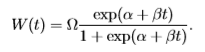
The origins of logistic regression can be traced back to the 19th century where it was created for describing both the growth rate of populations and the course of autocatalytic chemical reactions. Before the advent of logistic regression, the growth rate of some quantity W(t) – based on time t – would be represented as
Ŵ(t) = dW(t)/dt
where Ŵ(t) represents the rate of growth. The easiest assumption to make is that the rate of growth is proportional to the current population W(t):
Ŵ(t) = βW(t), β = Ŵ(t)/W(t)
with the constant rate of growth denoted as β.
If represented like so, though, the population increase would then grow exponentially. It was around the mid-19th century when Alphonse Quetelet, a Belegian statistician, and his pupil, Pierre-Francois Verhulst, decided to investigate the problem and make some adjustments. Verhulst initially approached the problem by adding an extra term to represent the increasing resistance to further growth towards the end as such:
Ŵ(t) = βW(t) - ϕ(W(t))
But after experimenting with a few additional terms, they were able to come up with a more representative equation that represents growth as being proportional to both the current population and the remaining room for growth:
The results were then published in 3 separate papers in the 1840’s in which the first paper actually illustrated how such a model accurately represented the population growth of France, Belgium, Essex, and Russia for various periods up to the 1830’s. There’s still a significant amount of detail leading up to the logistic regression model we have today, so please feel free to read more about it here.
Basic Concept

The plot above displays a sigmoid function, also known as a logistic function, which resembles an S-shaped curve and ensures that any values are mapped into some value between 0 and 1.
The logistic function can be mathematically represented as such:
1/(1+e-t)
where e is the base of natural logarithms and t represents the value you are attempting to transform.
How does all this relate to logistic regression though?
If you shift the terms in the equation above, you can form the one below:
y = (eb0+xb1)/(1+eb0+xb1)
where y is the predicted output that you want, b0 is the intercept term, and b1 is the coefficient for some input value x. If we relate the equation back to the earlier example, y would represent the probability that it will rain tomorrow whereas x could be the current temperature throughout the day. Keep in mind that, because the equation above was derived from the logistic function, the value y will always be between the values of 0 and 1 – which will represent the probability of our binary outcome occurring.
The formal representation of the logistic regression model is shown below:
To help make the concepts more concrete, let’s walk through an example.
The dataset I’ll be using this time is also from the UCI Machine Learning Repository and contains 303 instances of patients’ various attributes and whether they have heart disease or not. Below is a table that describes the 12 features referenced in the dataset:
Age
|
Age in years
|
Sex
|
(1 = male, 0 = female)
|
CP
|
Chest pain type (1-4)
|
TrestBPS
|
Resting blood pressure (in mm Hg)
|
Chol
|
Serum cholesterol in mg/dl
|
FBS
|
Fasting blood sugar > 120 mg/dl (1 = true; 0 = false)
|
Restecg
|
Resting electrocardiographic results (0-2)
|
Thalach
|
Maximum heart rate received
|
Exang
|
Exercise induced angina (1 = yes; 0 = no)
|
Oldpeak
|
ST depression induced by exercise relative to rest
|
Slope
|
Slope of the peak exercise ST segment (1-3)
|
import pandas as pd
import numpy as np
from sklearn.linear_model import LogisticRegression
from sklearn import metrics
import matplotlib.pyplot as plt
# read in data
my_data = pd.read_csv("heart_disease.csv")
# pre-processing the output value
my_data.loc[my_data['Output'] >= 1, 'Output'] = 1
The code snippet above imports the necessary libraries, reads in the csv file, and then preprocesses the output value so that it’s only either 0 or 1 (1 = heart disease; 0 = none).
For some reference on what the data looks like, I’ve included a snapshot of the first few rows:


class_means = my_data.groupby('Output').mean()
The above line of code groups the data by values in the “Output” column (so 0 and 1), and then calculates the mean value for each of the columns within each output value like so:
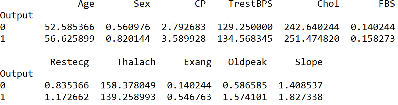
The above will help to give you a sense of what the data looks like. For instance, it seems that the average age of patients in the data is around the mid 50’s, and the resting blood pressure of the patients with heart disease looks to be, on average, higher than those without heart disease (in the TrestBPS column).
%matplotlib inline
pd.crosstab(my_data.Age, my_data.Output).plot(kind='bar')
plt.title('Heart Disease Frequency Based on Age')
plt.xlabel('Age')
plt.ylabel('Heart Disease Frequency')
plt.savefig('heart_disease_freq_age')
The code snippet above produces a cross-tabulation of the age and output values in the data and produces the following result:

It may be difficult to read the age values on the x-axis, but the general pattern is clear: older patients tend to be more likely to have heart disease than younger ones. This is merely one example of the types of exploratory data analysis we could do on the data beforehand to better understand what we’re dealing with and determine the best predictors for heart disease; there’s a lot more we can do, but I will leave the analysis at here for now.
# split y and x
y_train = my_data['Output']
my_data.drop('Output', axis=1, inplace=True)
# fit logistic regression model
my_log_model = LogisticRegression()
my_log_model.fit(my_data, y_train)
# creating test data dataframe
test_data = [
[60, 1, 1, 140, 240, 1, 0, 130, 0, 2.4, 3],
[20, 1, 1, 140, 240, 1, 0, 130, 0, 2.4, 2],
[10, 0, 1, 340, 440, 1, 0, 130, 0, 2.4, 2]
]
test_df = pd.DataFrame(test_data,columns=['Age','Sex', 'CP', 'TrestBPS', 'Chol', 'FBS', 'Restecg',
'Thalach', 'Exang', 'Oldpeak', 'Slope'])
The above code snippet splits the dataset into x-values and y-values before then fitting it all to a logistic regression model from the sci-kit learn package. To illustrate the results, I then create 3 rows of fake data for our fitted logistic regression model to predict values from.
# generating predictions
my_log_model.predict_proba(test_df)
my_log_model.predict(test_df)
The first line of the code snippet above produces the below values:
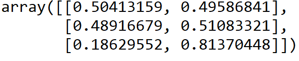
What do those mean? The values on the left represent the probability that the patient does not have heart disease, whereas the ones on the right represent the chances that he/she does – as a result, each row sums up to a value of 1.
When using logistic regression for classification, the most common cut-off for determining binary classes is 0.5, so in this case, the first patient would be predicted to not have heart disease whereas the second and third would have heart disease. Notice a difference though – the model predicted that the third patient would have an 81.37% chance of having heart disease, whereas the second patient would only have a 51.08% chance, which is significant. Rather than simply producing values of 0 or 1, logistic regression (due to its sigmoid function) can provide us information on how “close” some subject is to one of the class values.
As we’ve explained already, the logistic regression produces the below values for the patient classes:
Mathematical Details
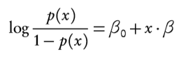
Formally, the logistic regression model is represented as:
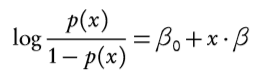
Where log(p/(1-p)) is known as a logistic (or logit) transformation.
How did statisticians come up with such a model? And why are we using the log odds? Odds, in this case, is represented by
p(x)/(1-p(x))
and is the ratio of the probability of the event divided by the probability of the complement of the event. For instance, let’s say the probability of raining tomorrow is 0.80. Therefore, the probability of not raining tomorrow is 0.20. The odds of raining tomorrow would then be
0.80 / (1 – 0.80) = 4
As a result, the odds of it raining tomorrow are 4 to 1. On the contrary, the odds of success are 1 to 1 if the probability of success if 0.50.
When working with logistic regression, statisticians are essentially attempting to model the conditional probability:
P(Y = 1 or 0|X = x) as a function of some x where the other parameters are estimated using the data
One obvious idea that we would need to incorporate into the model is some linearity with respect to x; some change in x would increment or decrement the probability by some amount, but there shouldn’t be any bounds to such values. Without any transformations, though, p(x) is bounded between the values of 0 and 1, so we clearly need some other method.
Below is a graph that you may see if you attempt to model a binary outcome using just the value of Y – not even the probability.
Although you can see above that higher values of x tend to contain more Y values of 0, the relationship isn’t linear and is hard to analyze.
What if we just use probability though? I mentioned earlier that probability by itself wouldn’t work due to its bounded nature, but below is a visualization:

Although the graph certainly looks a lot more linear (and having a sigmoidal shape) than the previous one using values of Y, its values are bounded.
An addition to using the probability of x, p(x), as the outcome would be to use log (x). Doing so would satisfy the characteristic of multiplying the outcome by some factor depending on the input variables, but the downside is that log is only unbounded in one direction.

There turns out to be multiple ways to model p(x) into an unbounded linear function – such as probit and square root of arcsin – but the easiest one to interpret turns out to be the logit transformation:
log(p/(1-p))
Let’s see exactly how easy it is to interpret the model using the logit transformation. Say we use the following example where we are predicting whether a patient has a cold or not, where the outcome is 1 for those with a cold and 0 for the others. Let’s say x1 = 0 for men and x1 = 1 for women.
Suppose we have the following:
log(p/(1-p)) = b0+b1x1
If we attempt to interpret the coefficients this way, the log odds of men having a cold would be equal to b0 whereas the log odds of women having a cold would be b0+b1x1.
If we then multiple both sides by e, we get:
p/(1-p) = eb0+b1x1
which can be interpreted as: the odds of having a cold are based on eb0+b1x1.
For men, the odds of having a cold is equal to eb0 whereas the odds of having a cold for women is eb0+b1x1.
If we then use some algebra to shift the values around, we can then get the following:
p=eb0+b1x1/(1+eb0+b1x1)
In this case, the probability that a man would have a cold is:
eb0/(1+eb0)
whereas the probability a woman could have a cold is:
eb0+b1x1/(1+eb0+b1x1)
So, although the results aren’t as simple as the additive factors from linear regression, using simple back-transformations on the logistic regression model significantly improve the model’s understandability.
In terms of terminology, the logit function on Y is known as the link function, which is essentially a function of the mean of the response variable Y that is used rather than merely the values of Y. In this case, we use the logit of Y as opposed to just 0 and 1 for binary classification.
Assumptions
Before even starting to model with logistic regression, though, it’s extremely important to check the data to see if it satisfies the following assumptions for logistic regression:
- Dependent variable is binary
- Observations are independent of each other
- Little or no multicollinearity among independent variables
- Linearity of independent variables and log odds
- Large sample size
First off, binary logistic regression requires that the dependent variable be binary – so with only two outcomes. Some categorical data sets may contain response variables that have more than two levels, such as the heart disease dataset I used in the first example. In those cases, you can simply verify the levels of the column in Python using:
my_data[‘output’].unique()
which will let you know the amount of unique values there are for that dependent variable. If there’s more than two, then simply combine various categories or just get rid of those rows.
The second assumption of logistic regression is a factor that’s also crucial for linear regression – independence among the observations. The easiest way to validate this would be to check exactly how the data was collected and whether there was any possibility of observations being correlated with each other during the collection process. For instance, let’s say I’m collecting data to model whether someone exercises or not. A lack of independence in observations in that case would be if I were to only collect data from groups of people I survey at the gym.
On a related note, it’s also crucial to check for little or no multicollinearity among the predictor variables – which is also expected for linear regression. Multicollinearity corresponds to the situation in which the data contains highly correlated independent variables; allowing it to be prevalent could hurt our ability to interpret the coefficients and analyze the model. Just as with linear regression, one commonly used method to detect multicollinearity is to use variance inflated factors, or VIF. As a rule of thumb, VIF values higher than 5 or 10 typically are causes for concerns.
One of the primary differences between linear and logistic regression occurs at the fourth assumption. For linear regression, linearity of independent variables and the response variable is assumed whereas the linearity of independent variables and the log odds of the response variable is the case for logistic regression. As I explained in the post on linear regression, a simple way to test for linearity is to plot the data and visualize it. In the case for logistic regression, though, we need to visualize the relationship between the log odds of Y versus X.
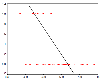
As I also showed earlier in this post, simply plotting the value of Y vs. X would lead to a plot like this:

(taken from http://thestatsgeek.com/2014/09/13/checking-functional-form-in-logistic-regression-using-loess/)
Visualizing such a plot is not very useful, unfortunately. You can probably see some general trend of X values, but it’s very hard to glean any more information than that. So, how can we improve it?
One way is to use a concept known as lowess/loess smoothing. A simplified version of general smoothing - not considered the lowess technique - plots a smoothed line of how the average value of Y changes with X by taking a running mean for each value of X and then joining them together. Lowess smoothing, on the other hand, is more complex and memory-intensive; it essentially fits a linear regression line around each value of X and joins them together to create the line. It inherently assumes linearity between Y and X, but only locally and not globally. If you’d like to read more about lowess smoothing, please feel free to find more information here.
An example of the above plot plotted using lowess smoothing is shown below:

(taken from http://thestatsgeek.com/2014/09/13/checking-functional-form-in-logistic-regression-using-loess/)
To then visualize the relationship between the log odds of Y and X, you would need to manually transform the probabilities from the lowess smoothing using the logit function.
Another way to test for the linearity assumption in logistic regression is with a Box-Tidwell Test for nonlinearity. I won’t go into the mathematic details of the Box-Tidwell Test here, but it essentially computes the best transformation of the predictor variables for you, if needed, for linearity. Below is an example of running the Box-Tidwell test on a model:
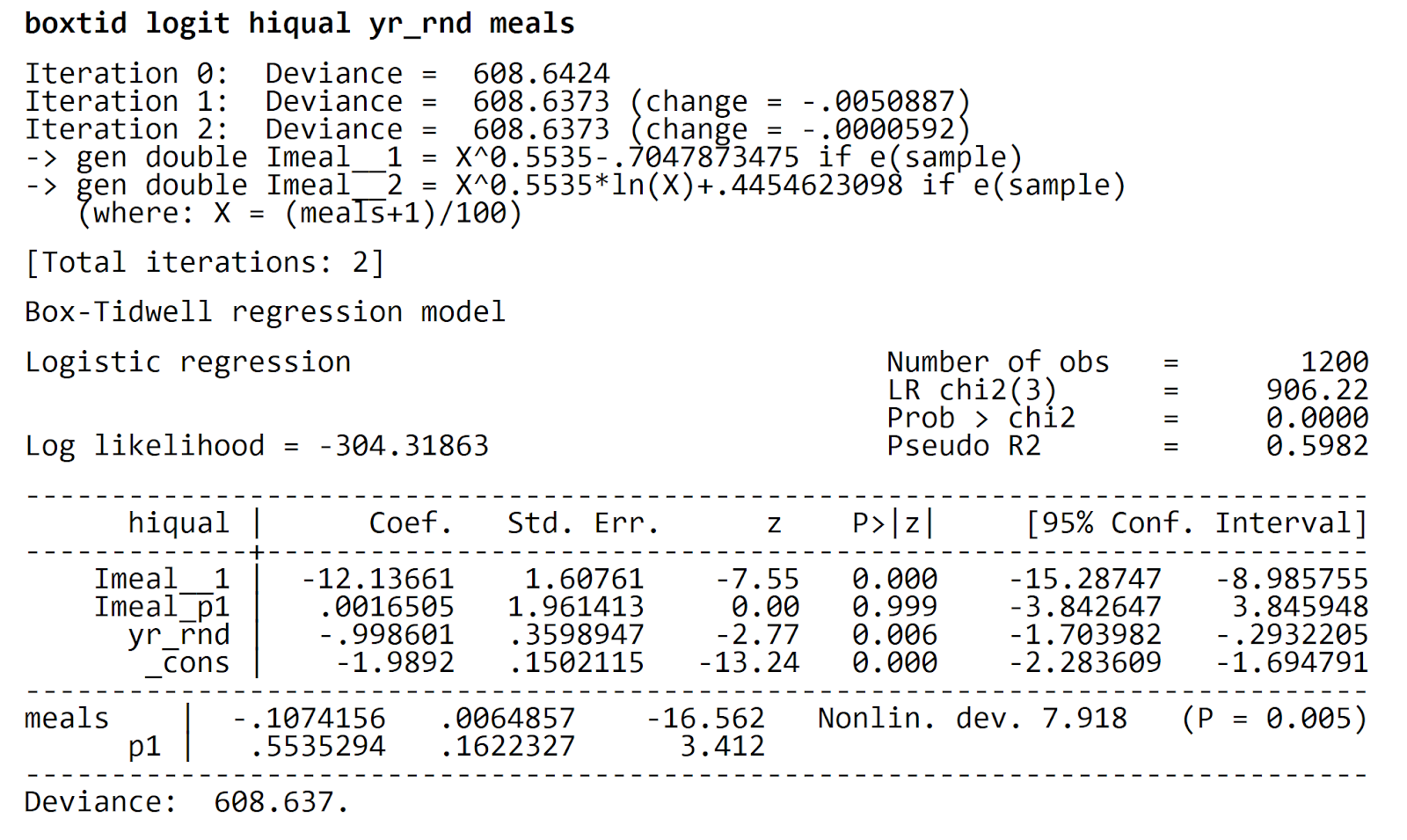
(taken from https://stats.idre.ucla.edu/stata/webbooks/logistic/chapter3/lesson-3-logistic-regression-diagnostics/)
In this example, “meals”, one of the predictor variables, is given a statistically significant p-value of .005 for the test of nonlinearity. The null hypothesis of the Box-Tidwell Test claims that the predictor variables “meals” is of a linear term, or with a “p1” value of 1, but in this case the test computes that a p1 value of .5535294 is optimal. As a result, transforming the “meals” predictor variable using a square-root function will help ensure linearity in this case.
Finally, the last assumption of logistic regression requires that you have a large sample size of data to work with. A useful guideline is that you need at least 10 observations with the least frequent outcome for each predictor variable in your model. For instance, if you have 10 predictor variables and the probability of your least frequent response variable is 0.10, then you’d need at least a sample size of:
(10 * 10) / (.10) = 1000
Model Evaluation
Now that all the logistic regression assumptions are met, and the model is built, how do you evaluate it? How do you know if your model is useful?
Here are some useful ways to measure your model’s performance:
- Observed probability vs. predicted probability graph
- Chi-squared Test of Goodness of Fit
- Confusion Matrix
- ROC Curve
If you prefer to visualize your data, the first method listed above may be useful for evaluating your model’s prediction power. You’ll first need to fit the logistic regression model to your data, run the model, and then save the predicted probabilities. You will then be able to plot your observed vs. predicted probabilities in a scatterplot; if the relationship is close to or is a straight line, then the predicted and observed probabilities are very similar which means your model is fitting the data very well. If the observed vs. predicted probabilities plot doesn’t turn out to be close to a straight line, you’ll need to adjust your model by adding more predictors, taking out useless ones, adding interactions, or with more other methods.
On a similar note, the Chi-squared Test of Goodness of Fit (also known as the Hosmer-Lemeshow X2 Test) determines whether sample data are consistent with a hypothesized distribution. In this case, we would compare the observed counts with the predicted counts for each group. The null and alternative hypotheses of the Chi-squared Test of Goodness of Fit are as follows:
Ho: The data are consistent with a specified distribution
Ha: The data are not consistent with a specified distribution
The test statistic for this is a Chi-squared Random Variable (X2) defined by the following equation:
X2 = ∑((Oi-Ei)2/Ei)
where Oi is the observed frequency count for group i and Ei is the expected frequency count. Using the test statistic, we would then calculate the p-value and determine whether to reject the null hypothesis based on that. In this case, we want for the p-value to be > .05 (depending on our confidence level) if we expect the model to predict our data well.
Yet another way to measure our logistic regression model’s performance is known as the confusion matrix, which is essentially a 2x2 matrix (or more depending on the number of classes) that contains counts for expected and actual results. An example is pictured below:
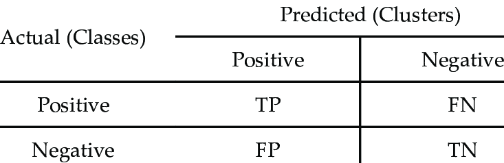
From the confusion matrix, we can gather many additional diagnostic measurements. Below is some terminology you should know:
True Positive (TP): We predicted yes and are correct
True Negative (TN): We predicted no and are correct
False Positive (FP): We predicted yes but are wrong (also known as Type 1 error)
False Negative (FN): We predicted no, but are wrong (also known as Type 2 error)
Each of those values can be gathered from the specified boxes as labeled in the confusion matrix shown above.
In addition to such values, we can also calculate the following rates:
Accuracy: How often is the classifier correct?
(TP + TN) / Total
Misclassification Rate: How often is it wrong?
(FP + FN) / Total
True Positive Rate: When an observation is actually positive, how often does the classifier predict positive?
TP / Actual Yes
False Positive Rate: When an observation is actually negative, how often does the classifier predict positive?
FP / Actual No
Specificity: When an observation is actually negative, how often does it predict negative?
TN / Actual No
Sensitivity: When an observation is actually positive, how often does it predict positive?
TP / Actual Yes
Precision: When the classifier predicts positive, how often is it correct?
TP / Predicted Yes
Prevalence: How often does the positive case occur in our sample?
Actual Yes / Total
There is a significant amount of metrics, but don’t feel overwhelmed since you most likely won’t need all of them; your choice of metric will primarily depend on your business objective. For instance, if you were creating a spam filter optimizing for precision may be best since you don’t want to keep sending actual e-mails into the spam folder accidentally.
Lastly, a way to visualize a lot of the measurements above is by using the Receiver Operating Characteristic Curve (ROC). With the ROC curve, you can more easily pick a threshold as well (rather than simply using 0.50 as the classification boundary) by checking the sensitivity and specificity at each point. A simple evaluation metric that you can also get from the ROC curve is the AUC, which is the percentage of the ROC plot that is underneath the curve. The AUC is a very useful single number summary of the classifier performance – the higher the better. If you’d like to learn more about the ROC curve and AUC values, feel free to read this.
Conclusion
Overall, the logistic regression model is in many ways very similar to linear regression albeit for classification purposes. Understanding the inner workings of logistic regression as well as its strengths and pitfalls will help greatly when learning about more powerful classifiers such as trees, random forests, and neural networks. Please feel free to look more into any of the resources I’ve used for additional details.
No comments:
Post a Comment