Abstract
In this report, I present my findings and experiences with the OpenAI Retro Contest (https://contest.openai.com/2018-1/) which was based on the Sonic the HedgehogTM video games. The experiments contained in this report are intended to assist other researchers with understanding the limitations and strengths of reinforcement learning. I also share multiple ideas that may be then fleshed out to provide boosts to agents playing video games.
1 Introduction
The primary goal of the contest, which was held from April 5 to June 5, 2018, was to create the best agent for playing unseen levels from the Sonic The Hedgehog video game series. The contest works in the following steps (as shown on the contest page [1]):
- Train or script your agent to play Sonic The Hedgehog
- Submit your agent as a Docker container
- Your agent will be evaluated on a set of custom-made test levels
- Your agent’s score will appear on the leaderboard
Submissions will be evaluated on 5 different test levels for a total of 1 million timesteps on each one. Timesteps refer to a set of 4 frames in the game; each step taken advances the Sonic game by 4 frames. On evaluation, each agent is essentially run for a variable number of episodes until the 1 million timesteps is reached. Each episode starts at the beginning of a level and concludes when either the agent dies, reaches the end of the level, or hits the timestep limit of 4,500 for an episode. The reward, or score, that you receive for your agent is proportional to its positive horizontal offset distance in each level - with a max reward of 9000 if you reach the end of the level. In addition to that, there is also a time bonus that starts at 1000 at the start of a level and decreases linearly to 0 by the end of the time limit [1].
For competitors starting out with the competition, OpenAI provided 3 different baseline algorithms: JERK, PPO, and Rainbow.
2 Algorithms
2.1 JERK Algorithm – “Just Enough Retained Knowledge”
The overall explanation of the JERK algorithm [2] is that it follows a scripted approach to advancing in the game, and then it gradually exploits more and more of the past actions that exhibited the greatest rewards towards the end.
The general algorithm for the baseline JERK algorithm goes as follows:
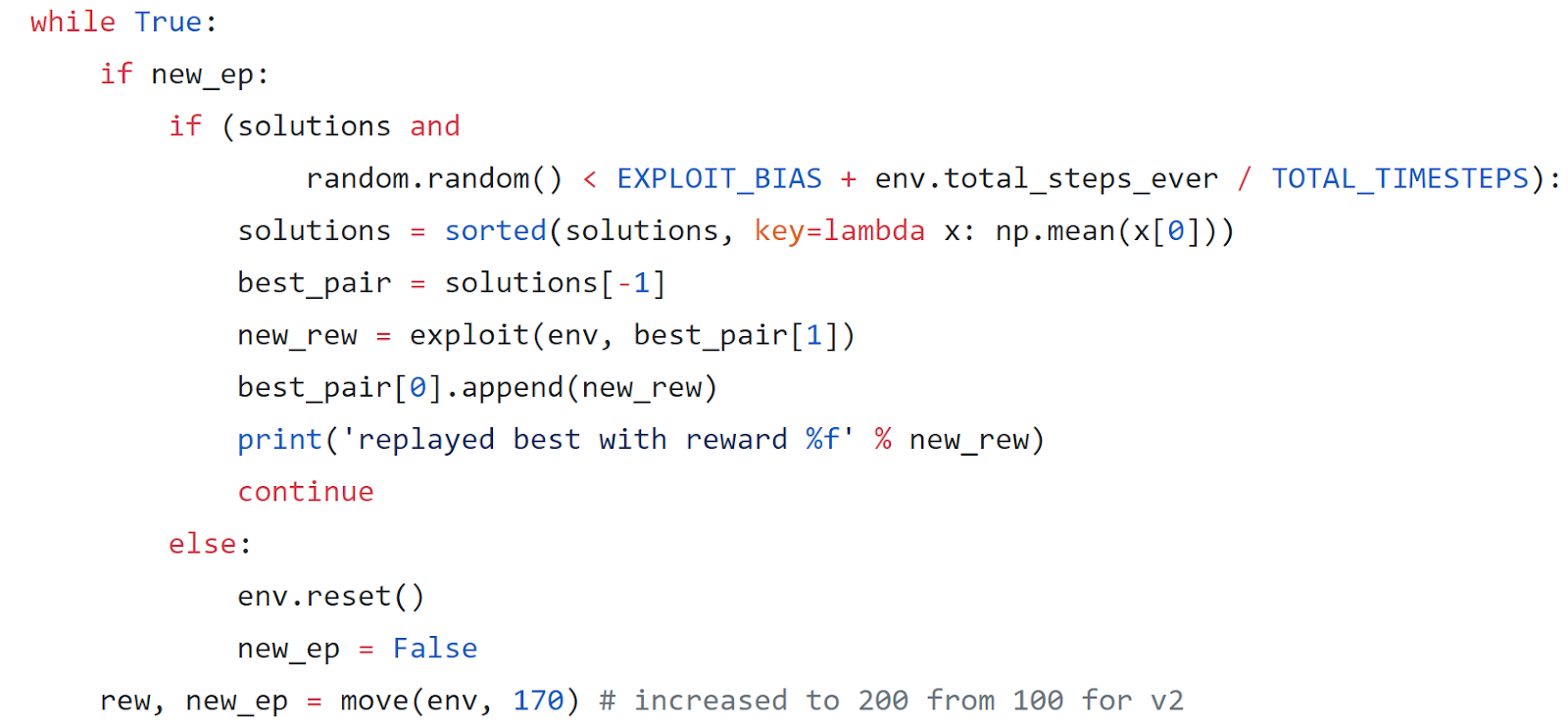
- If it’s not a new episode, exploit the best action sequence that has occurred so far with some probability that increases over time
- If it doesn’t exploit the best action sequence, then
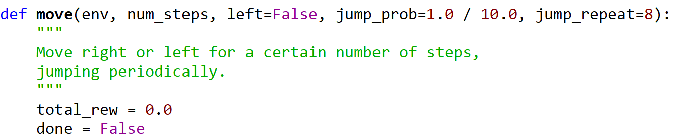
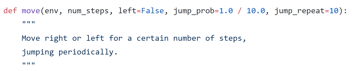
- Go right for 100 timesteps while doing 4 jumps in a row with a probability of 0.1
- If the total reward for going right was less than or equal to 0, then go left for 70 timesteps following the same pattern for jumping as going right
- Add the elapsed timesteps to a running count
- Repeat
Despite JERK’s simplicity, its scores proved to be higher than those of the other 2 baseline algorithms which I will cover after. The special pieces to note about the JERK algorithm are that it:
- Does not involve any sort of deep learning
- Does not consider any observations
- Only uses the reward to determine actions
2.2 Policy Gradient Algorithms
Before explaining the PPO algorithm, let me briefly cover the background of policy gradient algorithms [4]. Instead of attempting to act greedily on some value function like Q-learning algorithms do, policy gradient algorithms learn the actual policy itself. The policy can be thought of as the probability of taking a certain action given some state.
π=P(a|s)
To learn the policy, though, the model, with weights W, would take in state-action pairs and return the probabilities of taking an action A given some state S. Think of this being represented as:
π[w](s,a)
Given the gradient of the weights W for modifying the probability π, we can adjust the parameters in the direction while scaling based on the reward for the action.
Wt+1 = Wt + learningRate * [derivative of W to maximize P(a|s)] * [total reward]
The above formula [4] is a short example of how the policy gradient algorithm would learn using Monte-Carlo learning. The primary disadvantage of using Monte-Carlo learning is that the weights W are only updated at the end of each episode and, as a result, could produce a very high variance in results.
To combat such variance, another method known as actor-critic policy gradient learning can be used. The four main steps for actor-critic learning are as follows:
- Use π to estimate some value function V(s), the value of the current state
- Take some action based on the policy π
- Calculate the temporal-difference error of that action
- Update the parameters W while scaling with the temporal-difference error
TD Error = reward + discountFactor * V(next state) – V(current state)
The first 3 terms of the formula above [4], reward + discountFactor * V(next state) can be thought of as the value of taking some action A based on the current state. When subtracting the value of the current state from that, the temporal-difference error is essentially calculating the relative benefit of taking some action A when at the current state S. If the error is positive, then the action that was taken proved to be beneficial and vice-versa. On a related note, the magnitude of the error is also significant as it can greatly impact the amount by which the parameters W are adjusted.
2.3 Proximal Policy Optimization Algorithm
One of the baseline algorithms presented to us in the Retro Contest is the Proximal Policy Optimization algorithm [3], which essentially adds a few extra details to vanilla policy gradient algorithms. The primary difference is that the PPO algorithm attempts to update the policy, π, as conservatively as possible, without sacrificing its performance between policy updates. Other more advanced algorithms, such as TRPO, measure the amount of change in the policy between updates using a value known as the KL divergence, but PPO is able to simplify that even further by using a penalty term instead. With a concept similar to that of lasso and ridge regression, PPO clips the ratio of the new policy to the old policy to some value within a small range around 1.0 – where 1.0 means that the new and old policies are the same.
I won’t cover any of the mathematical details for the algorithms here, but feel free to look at [3] for more.
2.4 Q-learning Algorithms
Before going to the Rainbow algorithm, let’s also cover some brief details regarding Q-learning [5] in general. Vanilla Q -learning often uses matrices to represent the Q tables, where each row represents all the possible states and the columns represent all the possible actions; the values in the matrices are what we known as “Q values”. The higher the Q value, the more valuable that action is for the respective state.
How do we get the Q values? The Q value is obtained from the Q function, represented as:
Q(s, a)
which is the maximum expected future discounted reward possible if we take some action A from a given state S.
Q(s, a) = max E[rt + γrt+1 + γ2rt+2 + … | st = s, at = a, π]
The above equation [5] represents that the Q function for some state S and action A is the maximum sum of rewards rt discounted by γ for each timestep t.
The Q-learning algorithm essentially keeps repeating this step greedily until the episodes are over. To add in some exploration, though, a small probability of selecting a completely random action for some state S is often also assigned.
“Deep” Q-learning, on the other hand, merely uses deep learning techniques to represent the Q matrices. The neural network will take the observations of the current state in as inputs and then output the Q value as scalers for each of the possible actions at the end.
Ever since Deep Q Learning first came to existence, there have been several major improvements to the algorithm. I’ll discuss one of the major improvements here, but there are many more details that can be found [6].
One known problem with vanilla Q-learning was that it typically overestimated the Q-values of actions given some state S, which could easily result in non-optimal solutions. One solution to this was to decouple the two steps – choosing the next action and evaluating the possible actions. The primary neural network would then be used to select the action, whereas another secondary network would be solely used for predicting Q-values for each action. This improvement, known as Double DQN [6], from Hasselt et al. proved to significantly reduce the overestimation of Q-values and allowed the algorithms to train even faster.
2.5 Rainbow Algorithm
The Rainbow algorithm [6], on the other hand, essentially combines all of the individual major improvements that were made to DQN (Deep Q-learning) since it existed. The excellent paper which demonstrates that each of the improvements are actually complementary to each other provides significantly more detail [6].
More details on the baseline algorithms can be found [2].
3 Experiments
3.1 Initial Observations
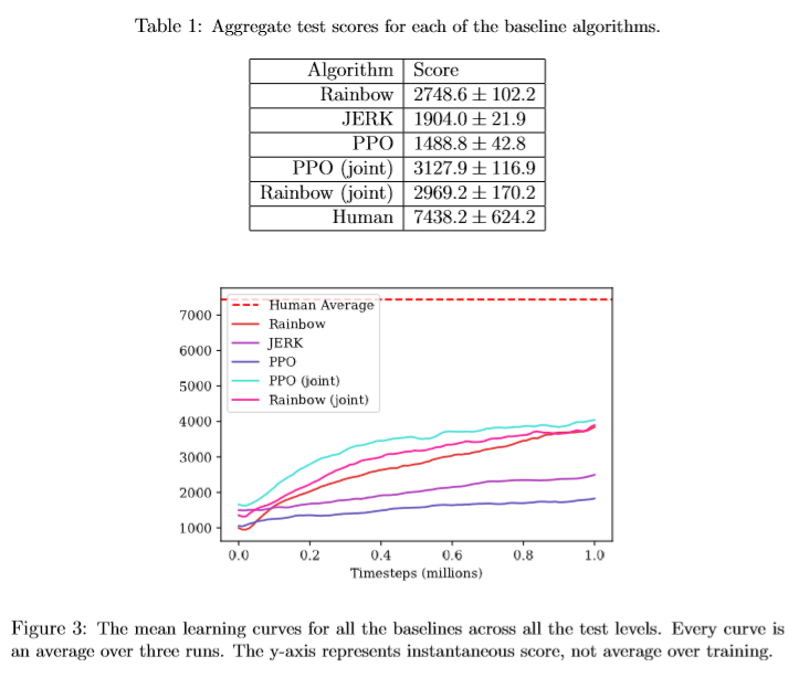
Before even running any experiments, I ensured that I read about each of the baseline algorithms in-depth and understood their performance values. According to [2], Joint PPO seems to be able to provide the highest test score for the lowest variance whereas Joint Rainbow may have a similar score with a higher variance. According to Table 1 in [2], it seems that training PPO on the training set provided the greatest boost when compared to the other two baseline algorithms. On the other hand, though, I was surprised to see that JERK didn’t seem to even compare to the other two baseline algorithms based on the results in the paper.
Despite Joint PPO and Rainbow seemingly producing high scores, all the baseline algorithms pale in comparison to a typical human-level score – which comes to about 7438 [2].
For reference, Table 1 and Figure 3 from the OpenAI paper are provided below [2]:
After having gathered those observations, I decided to first experiment with each of the baseline algorithms on my own before continuing more with one of them.
3.2 Experiments
From the start of the contest, OpenAI revealed to the contestants one of the test levels the algorithms would be evaluated against. Before going through my experiments, I’d like to specify what I refer to as the first four primary obstacles for Sonic on that level.
Obstacle 1:
This obstacle essentially consists of the two crab enemies that Sonic must somehow be able to get past.
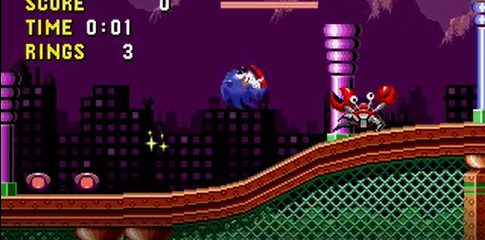
Obstacle 2:
This consists of the two spiked balls that Sonic must be able to traverse to cross.

Obstacle 3:
This consists of both the spring and the spinning blue enemy that Sonic must be able to use successfully and destroy to get to the next stage.

Obstacle 4:
This consists of a series of vertically moving blocks that Sonic must be able to traverse to get past.

3.3 Rainbow
Since the Rainbow baseline algorithm proved to score the best based on [2], it was one of the first ones that I tested for the Retro Contest.
Below are the results:
Table 2: Rainbow Algorithm Results
Run
|
Modifications
|
Score
|
1
|
Default
|
3795.86
|
2
|
Default
|
3265.56
|
Below are the recorded videos for the revealed evaluation level in the order of the table:
https://youtu.be/p4NLo2WQxTg (Run 1)
https://youtu.be/RZ3H5VLlVzI (Run 2)
Based on the video for Run 1, you can see that the baseline rainbow algorithm could potentially perform very well. It seemed to easily pass Obstacles 1, 2, and 3 with the two spiked balls and then smoothly used the spring to jump to the next level (0:00:11). It only seems that Sonic died where he did due to unfortunate chances since 1-2 additional steps to the left or the right at that point could have completely changed the outcome.
The video for Run 2 is very interesting though, and I believe it really highlights some of the pitfalls that even state-of-the-art DQN models experience. In the beginning of the run (up until about 0:00:15), you can see Sonic very easily crossing obstacles and even briefly reaching past where Run 2 did. To my surprise, though, Sonic then immediately starts going left, fails to process the correct action for getting to the next level with the spring at Obstacle 3, and then keeps going left. Interestingly, Sonic keeps going left until it gets to the area right before Obstacle 2 where it seems to process random actions – jumping up and down, staying still, running left/right. I noticed that at this point, Sonic seems to be unwilling to even get near or attempt getting past Obstacle 2 and instead just keeps pacing back and forth in the small area prior to Obstacle 2. A possible explanation would be that the Rainbow agent, based on past experiences, has learned that attempting to cross Obstacle 2 could lead to a decrease in score (due to hitting one of the spiked balls) and so, therefore, it just gets close to Obstacle 2 but then goes left again and repeats.
I personally thought the video for Run 2 was very enlightening as it really shines on the weaknesses that current reinforcement learning algorithms constantly experience.
To improve on the results, my initial thoughts would be to experiment with parameter tuning as “Students of Plato” (Rank 2) did according to [7]. It seems that tuning variables such as the batch size and target interval can significantly impact the Rainbow algorithm score albeit with a high variance as well.
3.4 PPO
After having tested the Rainbow algorithm, I then attempted with the PPO baseline algorithm (although only once).
Table 3: PPO Algorithm Results
Run
|
Modifications
|
Score
|
1
|
Default
|
2982.09
|
Below is the recorded video for the revealed test level for Run 1:
Surprisingly, the PPO algorithm seems to be rather shaky based on the video for Run 1. It crossed Obstacle 1 – albeit with some difficulty – and then even had wasted moments where it stayed still. Sonic was able to cross Obstacle 2 pretty easily but ultimately wasn’t even able to get to the location for Obstacle 3. Despite such results, I believe that this run turned out the way it did by unfortunate chance. For instance, when jumping off the ledge towards Obstacle 3, Sonic seemed to just jump a tad bit too early.
Initial thoughts for improvements would be to train PPO with various levels in the training set before the test server evaluations. I feel that, by exposing the PPO algorithm to many different types of levels, PPO can refine those minute details (such as when to jump off ledges) even more so that it can advance further in the test levels. “Students of Plato” also didn’t seem to advance PPO much further than a score of ~3.4k but that was without joint training as well [7].
Overall, my experiments with the PPO and Rainbow baseline algorithms were extremely limited due to time and computational resource constraints (especially since I found out about the competition rather late). If I were to do the competition again, I would definitely experiment more with the Rainbow algorithm and joint training, though, since it seemed to produce very strong results on its own already.
3.5 JERK
The baseline algorithm that I primarily experimented with for the duration of the competition was the JERK algorithm. Below are all the runs I’ve done with the JERK algorithm:
Table 4: JERK Algorithm Versions
Version
|
Modifications
|
1
|
Baseline
|
2
|
Right steps: 200
|
3
|
Right steps: 150
|
4
|
V3 and Exploit Bias: 0.40
|
5
|
V4 and Jump Repeat: 8
|
6
|
V5 and Jump Prob: 0.20
|
7
|
V5 and Spin Attack if not jumping
|
8
|
V7 modification
|
9
|
V5 and Go Right For Exploit-Waste
|
10
|
V9 and Right Steps: 170
|
11
|
V9 and Jump Repeat: 10
|
12
|
V9 and Spin Attack w/ Momentum: 7
|
13
|
V12 and Exploit-Waste as original move logic
|
14
|
V9 and Exploit-Waste as original move logic
|
15
|
V14 and (Spin Attack Prob., Momentum)
a: (0.3, 4)
b: (0.3, 7)
c: (0.3, 10)
d: (0.5, 4)
e: (0.5, 7)
f: (0.5, 10)
|
16
|
V14 and Exploit-Waste only go right
|
17
|
V14 and Spin Attack w/ Momentum 7 and Jump Next
|
18
|
V14 and Backtracking Reward: 50
|
19
|
V14 and Logic for manually checking for zero-reward
|
20
|
V19 and logic for cancelling future right jumps if negative reward
|
Table 5: JERK Algorithm Scores
Version
|
Run 1
|
Run 2
|
Run 3
|
Average Score
|
1
|
3815.14
|
-
|
-
|
3815.14
|
2
|
3688.94
|
3541.05
|
-
|
3614.995
|
3
|
3670.15
|
3847.55
|
3496.44
|
3671.38
|
4
|
3738.92
|
3854.28
|
3660.76
|
3751.32
|
5
|
3997.07
|
4068.99
|
4007.10
|
4024.387
|
6
|
3974.64
|
3930.06
|
3565.20
|
3823.3
|
7
|
3812.13
|
4155.07
|
3556.67
|
3841.29
|
8
|
3772.43
|
3672.70
|
3826.91
|
3757.347
|
9
|
4204.23
|
4237.60
|
4308.02
|
4249.95
|
10
|
4146.85
|
3934.01
|
3713.35
|
3931.403
|
11
|
4038.53
|
3896.52
|
3991.58
|
3975.543
|
12
|
3802.33
|
3767.77
|
3790.25
|
3786.783
|
13
|
3922.48
|
3748.94
|
3535.91
|
3735.777
|
14
|
3824.03
|
4370.99
|
4093.16
|
4096.06
|
15a
|
3701.67
|
3658.44
|
3684.85
|
3681.653
|
15b
|
4189.71
|
3955.28
|
3846.88
|
3997.29
|
15c
|
3721.44
|
3942.17
|
3818.58
|
3827.397
|
15d
|
3703.45
|
3641.93
|
-
|
3672.69
|
15e
|
3756.20
|
3837.06
|
-
|
3796.63
|
15f
|
3865.72
|
3943.05
|
3865.20
|
3891.323
|
16
|
4056.06
|
3933.83
|
4041.90
|
4010.597
|
17
|
3880.98
|
3743.26
|
3667.64
|
3763.96
|
18
|
4271.37
|
4090.07
|
4220.56
|
4194
|
19
|
4006.93
|
4056.50
|
-
|
4031.715
|
20
|
3645.80
|
3518.83
|
-
|
3582.315
|
Table 6: JERK Algorithm Highest Scores
Version
|
Task 1
|
Task 2
|
Task 3
|
Task 4
|
Task 5
|
Score
|
1
|
6593.67
|
2414.34
|
4945.70
|
2405.88
|
2716.11
|
3815.14
|
2
|
6200.51
|
2395.76
|
4598.48
|
2478.43
|
2972.12
|
3729.06
|
3
|
7672.43
|
2455.15
|
4350.82
|
2444.05
|
2894.78
|
3963.446
|
4
|
6569.28
|
2543.25
|
4599.01
|
2443.67
|
3212.38
|
3873.518
|
5
|
7674.53
|
2606.59
|
5311.72
|
2534.66
|
3071.66
|
4239.832
|
6
|
7365.34
|
2645.72
|
5206.88
|
2558.37
|
3247.05
|
4204.672
|
7
|
7745.98
|
2526.71
|
5275.76
|
2540.08
|
2720.44
|
4161.794
|
8
|
7134.13
|
2539.15
|
5074.41
|
2508.72
|
3038.08
|
4058.898
|
9
|
8093.04
|
2527.23
|
5378.94
|
2570.43
|
3213.42
|
4356.612
|
10
|
7804.06
|
2526.38
|
4952.72
|
2599.00
|
3206.56
|
4217.744
|
11
|
7003.51
|
3040.65
|
4823.49
|
2571.23
|
3200.63
|
4127.902
|
12
|
7383.66
|
3538.13
|
4412.90
|
3144.27
|
2194.87
|
4134.766
|
13
|
7310.30
|
3466.16
|
4344.23
|
2615.08
|
2506.63
|
4048.48
|
14
|
8036.30
|
2588.95
|
5555.53
|
2493.39
|
3270.96
|
4389.026
|
15a
|
6603.85
|
3347.11
|
4295.24
|
2599.39
|
2163.26
|
3801.77
|
15b
|
7721.88
|
3897.64
|
4548.08
|
3164.00
|
2623.69
|
4391.058
|
15c
|
7750.43
|
2782.12
|
4514.86
|
2535.27
|
2608.96
|
4038.328
|
15d
|
6659.66
|
3194.08
|
4148.11
|
3101.28
|
2145.15
|
3849.656
|
15e
|
6772.42
|
3377.92
|
4637.55
|
2454.88
|
2289.91
|
3906.536
|
15f
|
7610.29
|
2809.08
|
4880.04
|
2505.34
|
2444.12
|
4049.774
|
16
|
7862.97
|
2570.55
|
5049.26
|
2634.67
|
3052.18
|
4233.926
|
17
|
7437.64
|
3347.77
|
4349.54
|
2591.46
|
2563.75
|
4058.032
|
18
|
8499.60
|
2615.79
|
5016.43
|
2536.57
|
3104.05
|
4354.488
|
19
|
8000.27
|
2546.30
|
5226.51
|
2646.89
|
3203.42
|
4324.678
|
20
|
6747.10
|
2457.96
|
4347.13
|
2420.40
|
2669.54
|
3728.426
|
Version 1
This version simply consists of the baseline JERK algorithm as presented to us by OpenAI. Surprisingly, it scored higher than the baseline PPO and Rainbow algorithms right off the bat. Below is a sample video of its performance:
As you can see, Sonic does seem to struggle a bit crossing Obstacles 1 and 2 – getting hit multiple times. Compared to PPO and Rainbow, especially, Sonic’s movements through those first two obstacles definitely aren’t as smooth. The major problem with JERK, though, is Obstacle 3 – Sonic simply just gets stuck going back and forth with the spring for the rest of the episode. The reasoning behind that is probably due to JERK’s definitive nature and not having any sort of random actions that Sonic could try to get out of any endless loops. Despite seeing this, I decided to continue with improving JERK and actively brainstorming ways to avoid this endless loop at Obstacle 3.
Version 2
With this version, I simply increased the number of right steps that Sonic would take to be 200 from 100.
From the video it seems that JERK was able to move through Obstacle 2 more smoothly (without getting hit) but it still struggled with Obstacle 1 and ended up in a loop at Obstacle 3. Looking at the scores as well, the Version 2 changes actually seemed to decrease the overall score. A possible reason for that may be that the extra 100 steps going right may have misaligned with specific obstacles/platforms in the other test evaluation levels and thus caused Sonic to get stuck or die.
Version 3
This version was simply another experiment with the number of right steps that Sonic would take; I reduced it down to 150 from 200. Since most of the path that Sonic took in the provided test level video was the same, I won’t provide the video again, but Sonic did seem to be able to clear Obstacles 1 and 2 more easily without getting hit. Unfortunately, but as expected, Sonic still ends up in the loop at Obstacle 3. In terms of determining whether to continue with a version or not, I tended to use the highest single score as the decision-maker (in hindsight, I should have used a better metric); in this case, having the number of right steps at 150 seemed to provide the highest single-run score at 3847.55 compared to Version 1 and 2’s 3815.14 and 3688.94, respectively (taken from Table 5).
Version 4
For Version 4, I increased the probability of exploiting a past sequence from 0.25 to 0.40 and this, using my metric of single-run score, did prove to be better. I chose 0.40 because I wanted to increase Sonic’s likelihood of exploiting some past sequence – since we’re maintaining a running record of the best action sequence sin the past – but I didn’t want the probability so high that it would reduce the likelihood of Sonic discovering some new best sequence. 0.40 ended up being the value I chose, but I definitely would have experimented with multiple other values if I had more time.
In terms of the test level video provided, Sonic made it through Obstacles 1 and 2 but still ended up in the loop at Obstacle 3.
Version 5
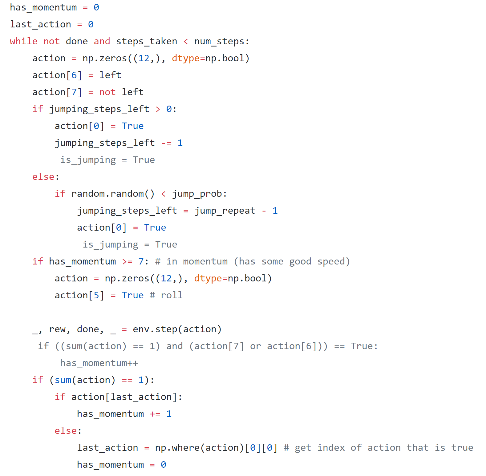
Perhaps the largest initial gain came from Version 5, where I simply increased the number of repeating jumps from 4 to 8. According to Table 5, the highest single-run score came out to be 4068.99 (first one higher than 4k!). A possible reason for such an increase may just be that jumping is good for Sonic. There aren’t too many scenarios where a jump would provide any disadvantage compared to Sonic running; in the case that Sonic jumps, he also spins so he is able to eliminate any enemies in his way that he would have hit otherwise. An exception would be if Sonic were to jump while going on some ramp (which would cause him to lose his momentum).
Despite the overall score increase, though, Sonic did seem to be shaky when overcoming Obstacles 1 and 2 and still ended up in the loop at Obstacle 3.
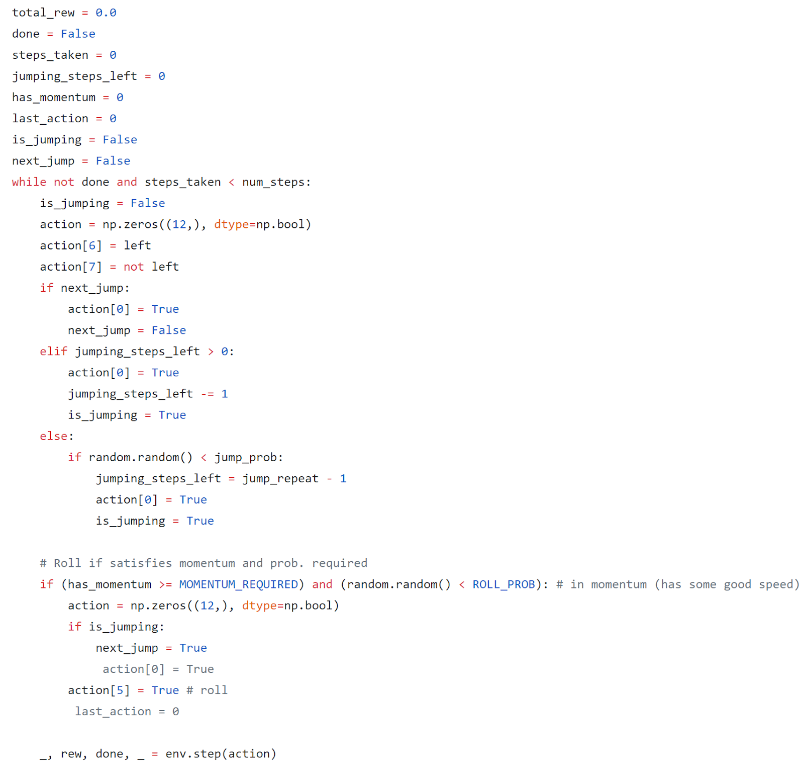
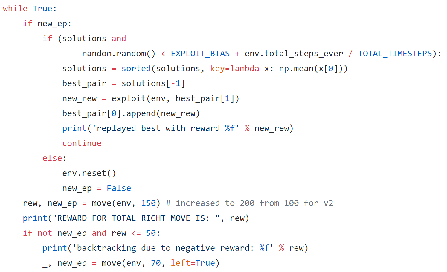
At this point, below are the relevant code snippets where I made the lasting changes so far:

Version 6
With this version, I simply increased the probability of jumping from 0.10 to 0.20. In doing so, the highest single-run score decreased from Version 5 and Sonic still ended up in the loop at Obstacle 3. An important note to remember is that, despite Sonic ending up in the loop for all these changes, Sonic is definitely experiencing different obstacles and reach points in the 4 other test levels so those ones are significantly affecting the overall score as well.
Versions 7 and 8
These 2 versions were both built on top of Version 5 and were also one of my initial attempts in adding a new move for Sonic – the spin attack (which is just pressing the down arrow with some momentum from right/left directions). My logic for doing so is that if Sonic were to keep running, then why not spin instead? By doing so, Sonic would still be moving forward while also eliminating any enemies in its path. On another note, I also watched the test level videos of top competitors and noted that one way for Sonic to cross Obstacle 3 is to actually spin while hitting the spring. Unfortunately, I realized only after testing both of these versions that my implementation for the spin attack was actually incorrect. As a result, please discard these two versions as anything but luck – despite reaching the high single-run score of 4155.07.
Version 9
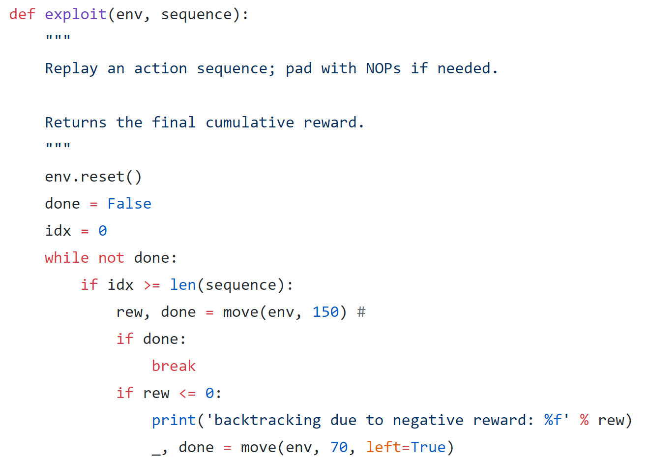
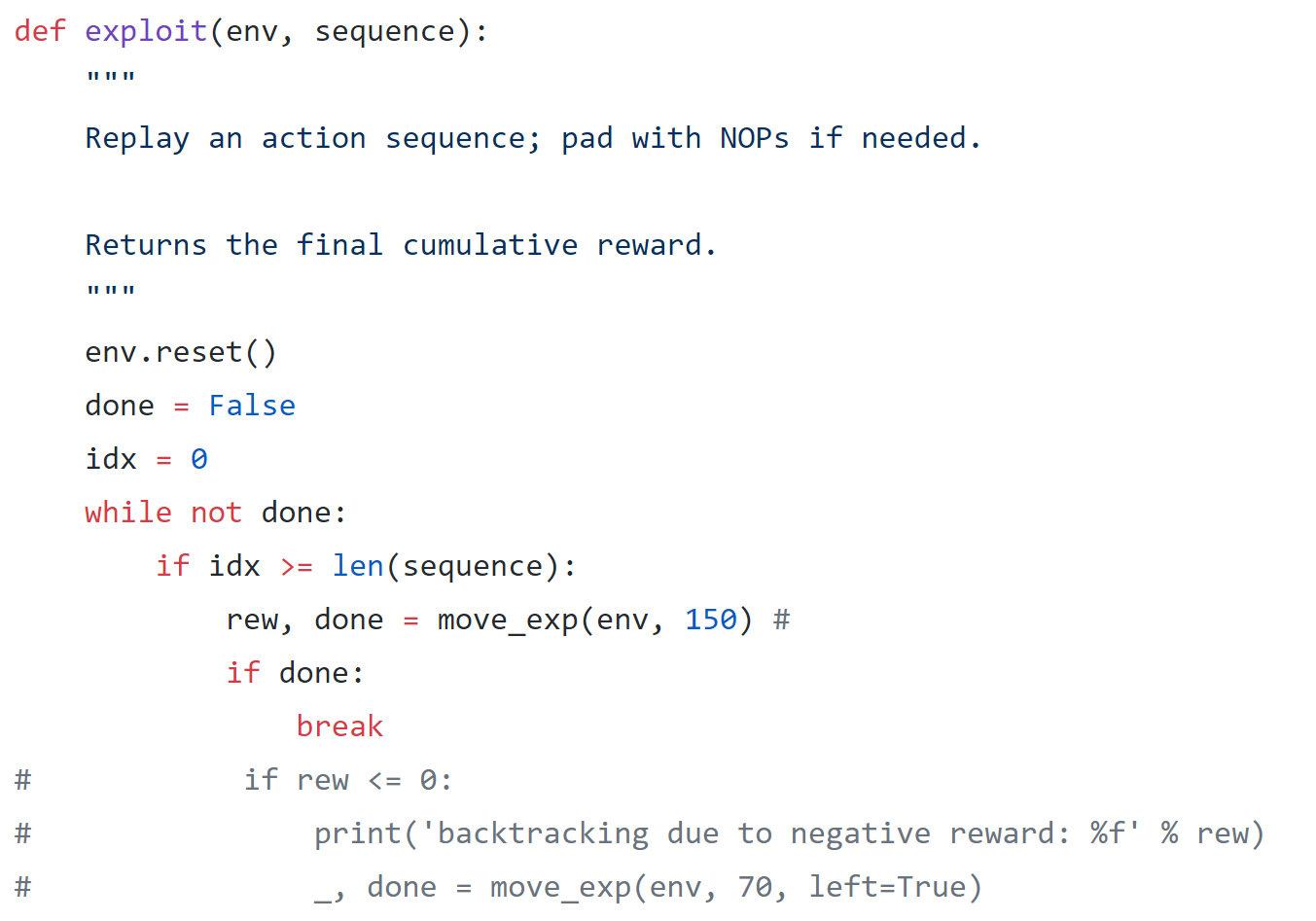
According to Table 4, I added “Go right for exploit-waste” in this version. By “exploit-waste”, I am referring to this condition in the exploit() function:

Before Version 9, Sonic essentially just stood at its current spot until the end of the episode once it used all of the actions in the previous best action sequence. In my opinion, Sonic would be wasting a massive amount of opportunity to gain even more distance if he just stood in the same spot. To test my initial hypothesis, I ran Sonic locally and added print statements if the above condition in the exploit() function were met, and I noticed that it happened quite frequently towards the end of later episodes.
As a result, I added the below snippet of code:

This modification proved to be enormous for the scores as Sonic was able to reach a single-run score of 4308.02 with the addition. Despite the significant score increase, Sonic still ends up in a loop at Obstacle 3; this time, though, Sonic didn’t seem to reach as high on the ramp at Obstacle 3. A possible reason might be that, by going right in the exploit() function, Sonic is facing the wrong way at the spring and therefore doesn’t gain as much right momentum.
Versions 10 and 11
For versions 10 and 11, I simply experimented a couple more times with modifying the number of right steps and repeating jumps that Sonic would take as shown below:
Version 10 -
Version 11 –
Neither of the changes produced any increases over the previous best single-run score of V9 though. One of my previous thoughts that “more jumping is always better” is definitely not logical according to these results. Again, these versions end up in the loop at Obstacle 3 but I’m sure some of the obstacles in the other test levels caused some trouble with these modifications.
Versions 12 and 13
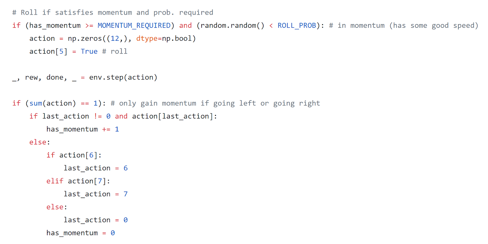
Built on top of version 9, version 12 adds the proper logic for producing the spin attack for Sonic as follows:
Version 13 then builds upon version 12 but adds the original move() as part of the exploit-waste piece in exploit() as below:
To my surprise, adding the logic for doing a spin attack in version 12 didn’t produce any notable increases over version 9. What was significant, though, was that Sonic was finally able to make it past Obstacle 3 based on the video below:
Despite getting significantly further in the single test level provided, Sonic’s overall single-run score did decrease though. You can possibly reason why based on how Sonic performs in Obstacles 1 and 2; Sonic seems to miss a lot of rings along its way and also sometimes seems to spin in the same position for no reason – pitfalls that I’m sure decrease Sonic’s performance drastically in the unseen test levels.
Version 13 seemed to still have a similar story to version 12, except I did notice that it seems to have immense trouble getting through the entirety of Obstacle 4 which makes sense considering the algorithmic nature of JERK.
Version 14
For version 14, I decided to remove the logic for the spin attack and just build on top of version 9 – the previous best one. I essentially added the logic from version 13 on top of version 9 and this is actually the version that produced the highest single-run score out of all versions: 4370.99.
Despite doing rather poorly on the provided test level (as can be seen in the video), the features from version 14 seemed to be able to perform highly on the other unseen levels instead. Another notable result is that version 14 produced the single highest run for task #3, according to Table 6 above.
Version 15
For version 15, I decided to test out various values for Sonic’s spin attack probability as well as momentum required like so:
The specific values I tested are in Table 4.
Perhaps the most notable one of all was version 15b with a probability of 0.3 and momentum required of 7; it produces a single-run score of 4189.71 (which didn’t surpass the 4370.99 from version 14) and actually resulted in the highest overall score for tasks #2 and 4. In hindsight, I could have possibly capitalized off of this and taken some logic from it to use in the future but I decided against that, at that moment, due to the single-run score value.
Version 16
In this version, I removed the option for Sonic to backtrack as part of the exploit-waste section in exploit() as below:
Such a change didn’t seem to produce any notable increases over version 14 (its base version) possibly due to the fact that if a series of right steps did produce a negative reward, going left to backtrack could actually prove to be beneficial for moving further right in the end.
Version 17
This version was an attempt to fix a problem I noticed in my logic from versions 12 and 15: when Sonic reaches the required momentum and spin attack probability, it heads straight to doing the spin attack and ignores any probability that it had for jumping that turn. I thought this could potentially make a massive difference since I could be greatly reducing the number of jumps that Sonic performs in a single episode by just cancelling them out like that.
As a result, I added in this logic for version 17 to fix it:
Unfortunately, though, the added modifications did nothing to boost the JERK algorithm’s score. Version 17 still is able to make it past Obstacle 3, but it’s hard to tell why the scores may be so much lower in the other unseen test levels. Sonic’s shakiness and trouble in clearing the first couple obstacles in the test level available could allude to some hints though.
Version 18
While evaluating my algorithms on various acts and zones locally, I noticed (from printing out rewards) that there are multiple cases where Sonic receives rewards around 10.0 or so after his initial series of right steps; so he receives a reward barely above the zero-mark but doesn’t end up making any real progress in the level. Despite barely making any progress and being stuck, Sonic doesn’t enter the condition for backtracking due to the positive reward and instead just keeps going at it over and over again. To fix this, I modified the reward boundary for backtracking to be 50 instead of 0 as shown below:
According to Table 5, the changes made here didn’t seem to produce anything higher than the scores of version 14 but that could just be due to luck. Given more time, I would definitely have experimented more with other values for the backtracking reward boundary, especially since it did produce the highest single-run score for task #1: 8499.60 according to Table 6.
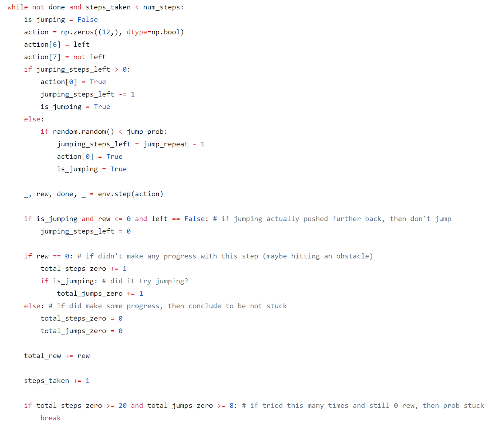
Versions 19 and 20
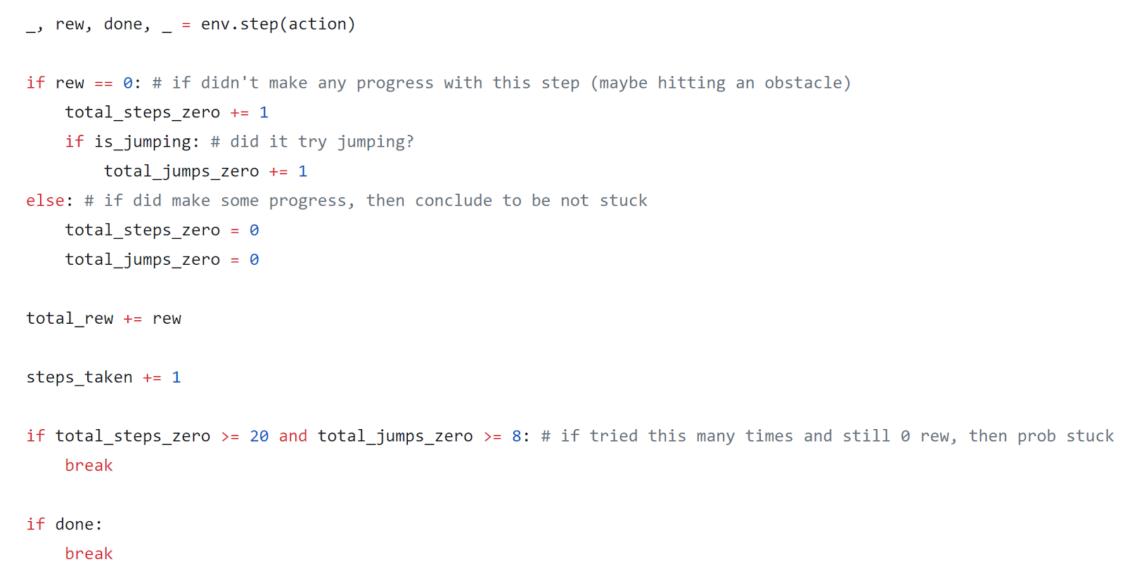
Based on Obstacle 4, I noticed that Sonic wastes a lot of timesteps in repeatedly trying to go one direction when it’s clearly stuck – and is probably hitting some wall or obstacle. That observation gave me the idea to actively check the number of times I’m getting zero reward from my steps, and once that number reaches a certain count, then I’ll simply cancel any additional steps in that same direction and instead backtrack or go the opposite direction. The logic can be seen below:
An additional piece, for version 20, that I decided to tack on was to cancel any future repeating jumps if the initial jumps actually resulted in a negative reward value. My reasoning behind this was that if Sonic decided to jump while climbing a ramp, then the jump would actually remove Sonic’s momentum and push him backwards, and thus removing his likelihood of clearing the ramp. I cancelled all future jumps if this even happened just once as in the code snippet below:
Despite thinking that such changes would reduce the amount of wasted moves significantly, the test runs from Table 5 proved me incorrect – with the single highest score coming out to be 4056.50. My best guess would be that such changes really only might play a beneficial effect in the visible test level (since that’s what I’m basing all my reasoning off of) but then actually significantly harm Sonic’s run in the unseen levels.
Overall, I intended for most of the modifications I made on the JERK algorithm to be as simple and generic as possible since I believed that if I were to add changes specific to special situations, then the algorithm may “overfit” onto a single test level.
4 Discussion
4.1 Possible Improvements
Due to major computational and time constraints, there were a lot of other experiments that I couldn’t carry out. Below I’ve listed some of the possible experiments I would’ve done barring the constraints:
- Testing additional values for the JERK parameters
Many of the versions that I had for JERK only tested 2-3 values for parameters such as the number of repeating jumps, and the probability for jumping and exploiting a past sequence. If I didn’t have the time constraint, I definitely would have experimented with additional values for each of those.
- Combine JERK with PPO/Rainbow
Towards the end of the competition, I had the idea of using PPO/Rainbow to solely predict when to jump whereas all the other logic would still follow what JERK does. My reasoning for this is that jumping is a significant action that could severely impact the end score and having a reinforcement learning algorithm predict when to jump based on the observations could theoretically provide a boost to the JERK algorithm scores.
- Tune the hyperparameters for PPO/Rainbow
“Students of Plato”, who ranked second in the competition, was able to get to that place solely through tuning the hyperparameters of the Rainbow baseline algorithm [7]. If I had more time, I definitely would try to experiment with that as well, especially since the baseline Rainbow algorithm already provides a strong score without any tuning.
- Add in joint training to PPO/Rainbow
Based on the research paper that OpenAI provided to us, it seems that joint training boosted the performance of all the reinforcement learning algorithms in every case. I’m very curious about what types of scores Rainbow would receive from the added transfer learning benefits; unfortunately, I wasn’t able to experiment with that due to computational resources.
- Test other reinforcement learning algorithms
Although Rainbow seems to be the reigning reinforcement learning algorithm for most cases now, I am very curious how some other algorithms – such as A2C, ACKTR, and ACER (which are also in the baselines repository) - might do on the Sonic video game series.
4.2 Conclusion
All in all, I’ve learned a tremendous amount about reinforcement learning from this contest. Coming into the competition, I had a strong machine learning experience from Kaggle competitions and undergraduate research but have never had any interactions with the reinforcement learning world. Having completed the contest in about the top 90th percentile, I can say that I’ve definitely gained a stronger understanding of reinforcement learning as well as an interest along with that. Please find my source code here: https://github.com/coded5282/OpenAI-Retro-Contest.
References
- “OpenAI Retro Contest.” OpenAI, contest.openai.com/
- Nichol, Alex, et al. Gotta Learn Fast: A New Benchmark for Generalization in RL. OpenAI, Gotta Learn Fast: A New Benchmark for Generalization in RL, s3-us-west-2.amazonaws.com/openai-assets/research-covers/retro-contest/gotta_learn_fast_report.pdf.
- Schulman, John, et al. Proximal Policy Optimization Algorithms. ArXiv, 2017, Proximal Policy Optimization Algorithms.
- Silver, David, et al. Deterministic Policy Gradient Algorithms. Deterministic Policy Gradient Algorithms, proceedings.mlr.press/v32/silver14.pdf.
- Mnih, Volodymyr, et al. Human-Level Control through Deep Reinforcement Learning. Nature, 2015, Human-Level Control through Deep Reinforcement Learning, storage.googleapis.com/deepmind-media/dqn/DQNNaturePaper.pdf.
- Hessel, Matteo, et al. Rainbow: Combining Improvements in Deep Reinforcement Learning. ArXiv, 2017, Rainbow: Combining Improvements in Deep Reinforcement Learning.
- Peter. OpenAI Retro Contest – Guide on “How to Score 6k Points on Leaderboard in AI Challange.” 2018, OpenAI Retro Contest – Guide on “How to Score 6k Points on Leaderboard in AI Challange,” www.noob-programmer.com/openai-retro-contest/how-to-score-6k-in-leaderboard/.